Stiffness#
Hydrogen-Oxygen Combustion Kinetics#
The combustion of hydrogen and oxygen can be described by a few elementary reactions, such as: 1. \(\text{H}_2 + O_2 \rightarrow 2OH \) 2. \(2OH \rightarrow H_2O + O \) 3. \(O + H_2 \rightarrow H + OH \) 4. \(H + O_2 \rightarrow O + OH \)
These reactions involve fast radical species (e.g., H, O, OH) and much slower species (e.g., H_2, O_2, H_2O). Due to the vastly different time scales (stiffness) between these reactions, a robust time integrator is required to accurately resolve the system over time.
System of Ordinary Differential Equations (ODEs)
The concentrations of species in this combustion reaction can be described by a system of coupled ODEs:
Let: • y_1 = [\text{H}_2] (concentration of hydrogen) • y_2 = [O_2] (concentration of oxygen) • y_3 = [\text{OH}] • y_4 = [H] • y_5 = [O] • y_6 = [H_2O]
Each species evolves over time based on the reaction rates and their current concentrations. A simplified set of ODEs might look like:
Where k_1, k_2, k_3, and k_4 are reaction rate constants for the four reactions. These rates may vary significantly, with some reactions being much faster than others, leading to stiffness in the equations.
# Re-import necessary libraries and redefine constants/functions after state reset
import numpy as np
import matplotlib.pyplot as plt
from scipy.integrate import solve_ivp
# Reaction rate constants (arbitrary units)
k1 = 0.2
k2 = 0.5
k3 = 0.1
k4 = 0.3
# System of ODEs for simplified combustion
def combustion_kinetics(t, y):
y1, y2, y3, y4, y5, y6 = y
dy1_dt = -k1 * y1 * y2 + k3 * y4 * y5
dy2_dt = -k1 * y1 * y2 + k4 * y4 * y2
dy3_dt = 2*k1 * y1 * y2 - k2 * y3**2 + k4 * y4 * y2
dy4_dt = -k3 * y4 * y5 + k4 * y4 * y2
dy5_dt = -k3 * y4 * y5 + k2 * y3**2
dy6_dt = k2 * y3**2
return [dy1_dt, dy2_dt, dy3_dt, dy4_dt, dy5_dt, dy6_dt]
# Initial concentrations (arbitrary units)
y0 = [1.0, 1.0, 0.0, 0.0, 0.0, 0.0] # [H2, O2, OH, H, O, H2O]
# Time points
t_eval = np.linspace(0, 10, 1000)
# Solve the ODEs using an explicit method (RK45) and implicit method (BDF)
sol_explicit = solve_ivp(combustion_kinetics, [0, 10], y0, method='RK45', t_eval=t_eval)
sol_implicit = solve_ivp(combustion_kinetics, [0, 10], y0, method='BDF', t_eval=t_eval)
# Define a function to compute the Jacobian matrix of the system at any point
def jacobian(y):
y1, y2, y3, y4, y5, y6 = y
J = np.zeros((6, 6))
# Partial derivatives for each species with respect to each other
J[0, 0] = -k1 * y2
J[0, 1] = -k1 * y1
J[0, 3] = k3 * y5
J[0, 4] = k3 * y4
J[1, 0] = -k1 * y2
J[1, 1] = -k1 * y1 + k4 * y4
J[1, 3] = k4 * y2
J[2, 0] = 2 * k1 * y2
J[2, 1] = 2 * k1 * y1
J[2, 2] = -2 * k2 * y3
J[2, 3] = k4 * y2
J[3, 3] = -k3 * y5 + k4 * y2
J[3, 4] = -k3 * y4
J[4, 3] = -k3 * y5
J[4, 4] = -k3 * y4 + 2 * k2 * y3
J[5, 2] = 2 * k2 * y3
return J
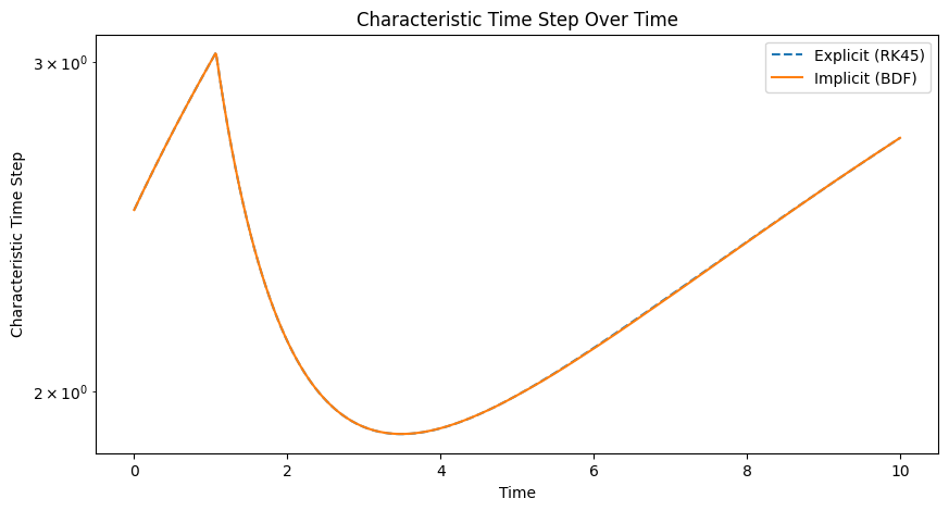
# Calculate the characteristic time step as the inverse of the largest eigenvalue
def characteristic_time_step(y):
J = jacobian(y)
eigenvalues = np.linalg.eigvals(J)
max_eigenvalue = np.max(np.abs(eigenvalues))
return 1 / max_eigenvalue if max_eigenvalue != 0 else np.inf
# Compute characteristic time steps along the solution
time_steps_explicit = [characteristic_time_step(y) for y in sol_explicit.y.T]
time_steps_implicit = [characteristic_time_step(y) for y in sol_implicit.y.T]
# Plot the characteristic time step over time for both methods
plt.figure(figsize=(10, 5))
plt.plot(sol_explicit.t, time_steps_explicit, label='Explicit (RK45)', linestyle='--')
plt.plot(sol_implicit.t, time_steps_implicit, label='Implicit (BDF)')
plt.yscale('log')
plt.xlabel('Time')
plt.ylabel('Characteristic Time Step')
plt.title('Characteristic Time Step Over Time')
plt.legend()
plt.show()
import numpy as np
import matplotlib.pyplot as plt
from scipy.integrate import solve_ivp
# Reaction rate constants (arbitrary units)
k1 = 0.2
k2 = 0.5
k3 = 0.1
k4 = 0.3
# System of ODEs for simplified combustion
def combustion_kinetics(t, y):
y1, y2, y3, y4, y5, y6 = y
dy1_dt = -k1 * y1 * y2 + k3 * y4 * y5
dy2_dt = -k1 * y1 * y2 + k4 * y4 * y2
dy3_dt = 2*k1 * y1 * y2 - k2 * y3**2 + k4 * y4 * y2
dy4_dt = -k3 * y4 * y5 + k4 * y4 * y2
dy5_dt = -k3 * y4 * y5 + k2 * y3**2
dy6_dt = k2 * y3**2
return [dy1_dt, dy2_dt, dy3_dt, dy4_dt, dy5_dt, dy6_dt]
# Initial concentrations (arbitrary units)
y0 = [1.0, 1.0, 0.0, 0.0, 0.0, 0.0] # [H2, O2, OH, H, O, H2O]
# Time points
t_eval = np.linspace(0, 10, 1000)
# Solve the ODEs using an explicit method (RK45)
sol_explicit = solve_ivp(combustion_kinetics, [0, 10], y0, method='RK45', t_eval=t_eval)
# Solve the ODEs using an implicit method (BDF)
sol_implicit = solve_ivp(combustion_kinetics, [0, 10], y0, method='BDF', t_eval=t_eval)
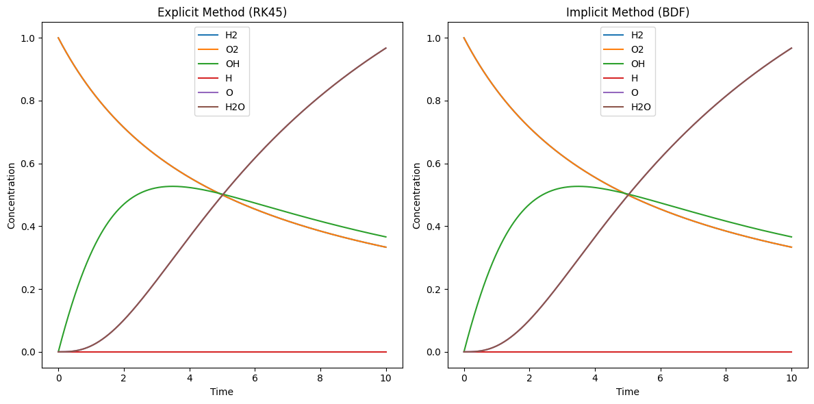
# Plot the results
plt.figure(figsize=(12, 6))
# Plot for Explicit method (RK45)
plt.subplot(1, 2, 1)
plt.plot(sol_explicit.t, sol_explicit.y[0], label='H2')
plt.plot(sol_explicit.t, sol_explicit.y[1], label='O2')
plt.plot(sol_explicit.t, sol_explicit.y[2], label='OH')
plt.plot(sol_explicit.t, sol_explicit.y[3], label='H')
plt.plot(sol_explicit.t, sol_explicit.y[4], label='O')
plt.plot(sol_explicit.t, sol_explicit.y[5], label='H2O')
plt.title('Explicit Method (RK45)')
plt.xlabel('Time')
plt.ylabel('Concentration')
plt.legend()
# Plot for Implicit method (BDF)
plt.subplot(1, 2, 2)
plt.plot(sol_implicit.t, sol_implicit.y[0], label='H2')
plt.plot(sol_implicit.t, sol_implicit.y[1], label='O2')
plt.plot(sol_implicit.t, sol_implicit.y[2], label='OH')
plt.plot(sol_implicit.t, sol_implicit.y[3], label='H')
plt.plot(sol_implicit.t, sol_implicit.y[4], label='O')
plt.plot(sol_implicit.t, sol_implicit.y[5], label='H2O')
plt.title('Implicit Method (BDF)')
plt.xlabel('Time')
plt.ylabel('Concentration')
plt.legend()
plt.tight_layout()
plt.show()
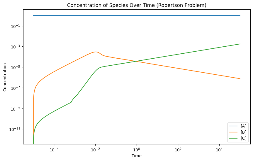
## Robertson (1966)
# Define rate constants for the Robertson problem (1966)
k1 = 0.04
k2 = 1e4
k3 = 3e7

# Define the ODE system for Robertson's reaction mechanism
def robertson_kinetics(t, y):
    """Robetson's reaction mechanism ODE system.
        k1: A -> B
        k2: 2B -> C + B
        k3: B + C -> A + C
    Args:
        t (_type_): _description_
        y (_type_): _description_

    Returns:
        _type_: change rate
    """
    A, B, C = y
    dA_dt = -k1 * A + k3 * B*C
    dB_dt = k1 * A - k2 * B**2 - k3 * B*C
    dC_dt = k2 * B**2
    return [dA_dt, dB_dt, dC_dt]

# Initial concentrations (arbitrary units)
y0 = [1.0, 0.0, 0.0]  # [A, B, C]

# Time points for evaluation
t_eval = np.logspace(-5, 5, 1000)  # From 1e-6 to 10 (log scale)

# Solve the ODEs using the implicit method (BDF) for stability with stiff system
sol_robertson = solve_ivp(robertson_kinetics, [t_eval[0], t_eval[-1]], y0, method='BDF', t_eval=t_eval)

# Plot the concentrations over time
plt.figure(figsize=(10, 6))
plt.plot(sol_robertson.t, sol_robertson.y[0], label='[A]')
plt.plot(sol_robertson.t, sol_robertson.y[1], label='[B]')
plt.plot(sol_robertson.t, sol_robertson.y[2], label='[C]')
plt.yscale('log')
plt.xscale('log')
plt.xlabel('Time')
plt.ylabel('Concentration')
plt.title('Concentration of Species Over Time (Robertson Problem)')
plt.legend()
plt.show()
# Redefine the Jacobian function for Robertson's problem
def robertson_jacobian(y):
    A, B, C = y
    J = np.zeros((3, 3))

    # Partial derivatives for each species with respect to each other
    J[0, 0] = -k1
    J[0, 2] = k3
    J[1, 0] = k1
    J[1, 1] = -2 * k2 * B
    J[2, 1] = 2 * k2 * B
    J[2, 2] = -k3

    return J

# Calculate the characteristic time step as the inverse of the largest eigenvalue
def characteristic_time_step_robertson(y):
    J = robertson_jacobian(y)
    eigenvalues = np.linalg.eigvals(J)
    max_eigenvalue = np.max(np.abs(eigenvalues))
    return 1 / max_eigenvalue if max_eigenvalue != 0 else np.inf

# Compute characteristic time steps along the solution (only for the BDF solution)
time_steps_implicit_robertson = [characteristic_time_step_robertson(y) for y in sol_implicit_robertson.y.T]

# Plot the characteristic time step over time for the BDF method
plt.figure(figsize=(8, 5))
plt.plot(sol_implicit_robertson.t, time_steps_implicit_robertson, label='Implicit (BDF)')
plt.yscale('log')
plt.xscale('log')
plt.xlabel('Time')
plt.ylabel('Characteristic Time Step')
plt.title('Characteristic Time Step Over Time (Robertson Problem, BDF)')
plt.legend()
plt.show()
---------------------------------------------------------------------------
NameError                                 Traceback (most recent call last)
Cell In[5], line 24
     21     return 1 / max_eigenvalue if max_eigenvalue != 0 else np.inf
     23 # Compute characteristic time steps along the solution (only for the BDF solution)
---> 24 time_steps_implicit_robertson = [characteristic_time_step_robertson(y) for y in sol_implicit_robertson.y.T]
     26 # Plot the characteristic time step over time for the BDF method
     27 plt.figure(figsize=(8, 5))

NameError: name 'sol_implicit_robertson' is not defined