ROW and Gauss-Legendre implicit method

import numpy as np
import matplotlib.pyplot as plt

# Define a sample nonlinear system of ODEs for testing
def nonlinear_system(t, y):
    return np.array([y[1], -y[0] + 0.1 * y[0] * (1 - y[0]**2)])

def row2_step(f, t, y, h):
    """Performs a single integration step using ROW2 method."""
    # ROW2 Butcher coefficients
    a21 = 1 / (2 - np.sqrt(2))
    b1 = 1 / (2 - np.sqrt(2))
    b2 = 1 - b1

    # Calculate intermediate steps
    k1 = f(t, y)
    k2 = f(t + h / (2 - np.sqrt(2)), y + h * a21 * k1)
    
    # Update solution
    y_next = y + h * (b1 * k1 + b2 * k2)
    return y_next

def gauss_legendre_step(f, t, y, h):
    """Performs a single integration step using the two-stage Gauss-Legendre method."""
    # Gauss-Legendre coefficients for 2-stage method
    c1 = 0.5 - np.sqrt(3) / 6
    c2 = 0.5 + np.sqrt(3) / 6
    a11 = 0.25
    a12 = 0.25 - np.sqrt(3) / 6
    a21 = 0.25 + np.sqrt(3) / 6
    a22 = 0.25
    b1 = 0.5
    b2 = 0.5

    # Initial guesses for k1 and k2
    k1 = f(t + c1 * h, y)
    k2 = f(t + c2 * h, y)
    
    # Fixed-point iteration (or nonlinear solver) would be used here for a real implicit method.
    for _ in range(5):  # Iterate to refine k1 and k2
        k1 = f(t + c1 * h, y + h * (a11 * k1 + a12 * k2))
        k2 = f(t + c2 * h, y + h * (a21 * k1 + a22 * k2))
    
    # Update solution
    y_next = y + h * (b1 * k1 + b2 * k2)
    return y_next

# Set initial condition, time step, and time range
y0 = [1.0, 0.0]  # Initial values
t0 = 0.0
tf = 20.0
h = 0.01
n_steps = int((tf - t0) / h)

# Prepare storage for results
t_values = [t0]
y_values_row2 = [y0]
y_values_gauss = [y0]

# Perform integration using ROW2 and Gauss-Legendre
y_row2 = np.array(y0)
y_gauss = np.array(y0)
t = t0

for _ in range(n_steps):
    y_row2 = row2_step(nonlinear_system, t, y_row2, h)
    y_gauss = gauss_legendre_step(nonlinear_system, t, y_gauss, h)
    
    t += h
    t_values.append(t)
    y_values_row2.append(y_row2)
    y_values_gauss.append(y_gauss)

# Convert results to arrays for plotting
t_values = np.array(t_values)
y_values_row2 = np.array(y_values_row2)
y_values_gauss = np.array(y_values_gauss)

# Plot the results
plt.figure(figsize=(10, 6))
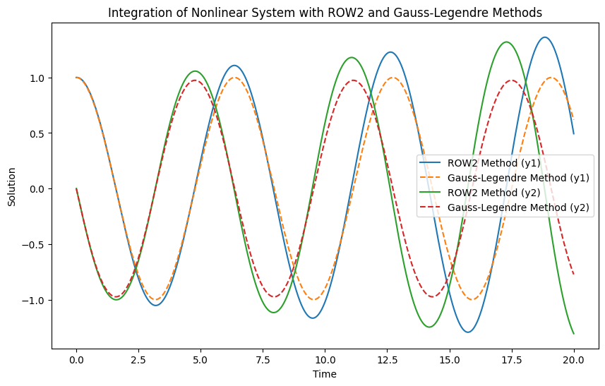
plt.plot(t_values, y_values_row2[:, 0], label='ROW2 Method (y1)')
plt.plot(t_values, y_values_gauss[:, 0], label='Gauss-Legendre Method (y1)', linestyle='--')
plt.plot(t_values, y_values_row2[:, 1], label='ROW2 Method (y2)')
plt.plot(t_values, y_values_gauss[:, 1], label='Gauss-Legendre Method (y2)', linestyle='--')
plt.xlabel('Time')
plt.ylabel('Solution')
plt.title('Integration of Nonlinear System with ROW2 and Gauss-Legendre Methods')
plt.legend()
plt.show()