Spectral discretization#
A spectral discretization uses a basis of functions which dimension is the maximum order of representation of a solution. In an spectral collocation method, the variables are the values at N collocation points. The expected error is then proportional to \((1/N)^N\) unlike classical p-order methods whose error is proportional to \((1/N)^p\).
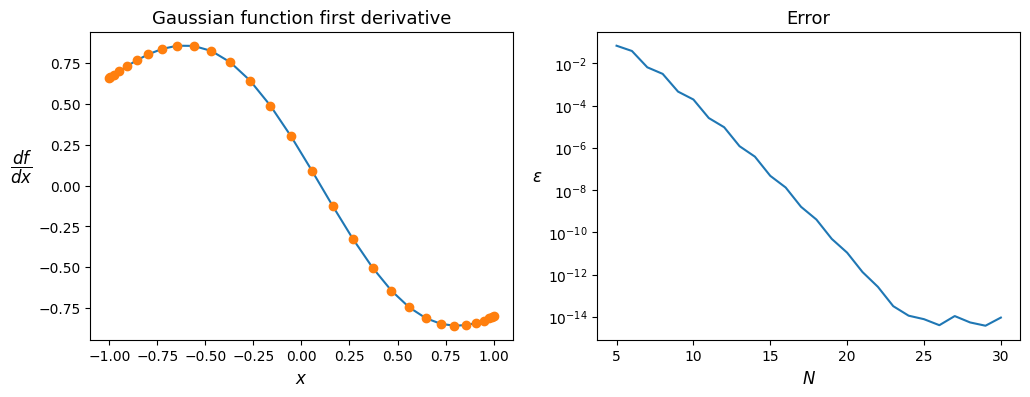
To analyze the convergence, a function f is discretized on collocation points. The derivated function is computed thanks to the differentiation operator and compared to the theoretical function.
import numtoolkit.spectral as sp
import numpy as np

def f(x):
    return np.exp(-((x - 0.1) ** 2))

def df(x):
    return -2 * (x - 0.1) * f(x)

def df2(x):
    return -2 * (1 - 2.*(x - 0.1)**2) * f(x)
Validation of Chebyshev derivation operator#
Discretized (using matrix vector product) and theoretical first and second order deratives are compared.
import matplotlib.pyplot as plt
plt.rcParams.update({"axes.labelsize":12, "axes.titlesize":13 })
#
alln = range(5,31) # mesh sizes
err = np.zeros(len(alln))
#
for i, n in enumerate(alln):
  SpOp = sp.ChebCollocation(n)
  x = SpOp.x # collocation points
  df_th = df(x)
  df_num = SpOp.matder(1) @ f(x)
  err[i] = np.sqrt(np.sum((df_th-df_num)**2)/n )

fig, (ax1, ax2) = plt.subplots(1, 2, figsize=(12,4))
ax1.plot(x, df_th, '-', x, df_num, 'o')
ax1.set_title('Gaussian function first derivative')
ax1.set_xlabel('$x$')
ax1.set_ylabel('$\dfrac{{d} f}{{d} x}$',rotation='horizontal', ha='right')
ax2.set_title('Error')
ax2.semilogy(alln, err)
ax2.set_xlabel('$N$')
ax2.set_ylabel('$\epsilon$',rotation='horizontal', ha='right');
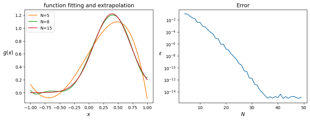
Curve fitting#
Assuming the continuous function is not known, only a (often continuous) sampling is offered. Since Chebyshev collocation methods prefer using their own collocation points. It is recommended to fit Chebyshev at these points (non linear mapping are not yet available there, V1.2.1).
g = lambda x: np.exp(-5*(x-.2)*(x-.6))
x_uni = np.linspace(-1, 1, 101, endpoint=True)
samples = g(x_uni)
#
# param plot
fig, (ax1, ax2) = plt.subplots(1, 2, figsize=(12,4))
ax1.set_title('function fitting and extrapolation')
ax1.set_xlabel('$x$')
ax1.set_ylabel('$g(x)$',rotation='horizontal', ha='right')
ax1.plot(x_uni, samples)
ax2.set_title('Error')
ax2.set_xlabel('$N$')
ax2.set_ylabel('$\epsilon$',rotation='horizontal', ha='right');
#
alln = np.arange(4, 50)
plotn = (5, 8, 15)
err = np.zeros((len(alln)))
for i, n in enumerate(alln):
    SpOp = sp.ChebCollocation(n)
    f_xi = SpOp.fit_to_gauss(x_uni, samples)
    newf = SpOp.extrapol(f_xi, x_uni)
    err[i] = np.sqrt(np.sum((newf-samples)**2)/samples.size )
    if n in plotn:
        ax1.plot(x_uni, newf, label=f"N={n}")
        ax1.legend()
#
ax2.semilogy(alln, err)
[<matplotlib.lines.Line2D at 0x7f3b7e5cc650>]