Upwind and Central scheme

%matplotlib inline
import numpy as np
import matplotlib.pyplot as plt

On cherche à résoudre l’évolution instationnaire du problème linéaire de convection suivant

\[ \frac{\partial q}{\partial t} + a \frac{\partial q}{\partial x} = 0 \]

pour la quantité transportée \(q(x,t)\) et la condition intiale \(q_0(x)\) sur le domaine \([0;\ell]\) avec des conditions périodiques. On choisit \(\ell=1\rm~m\) et \(a=1\rm~m/s\).

ndof  = 100
xi    = np.linspace(0,1,ndof+1)  # grid definition
aconv = 1.0                      # Advection velocity

def qinit(x):                 # Initial condition
    q0 = np.exp(-200.*(x-0.3)**2)
    # q0 = .5+.5*np.sin(2*x*np.pi)
    # q0 = .5+.5*np.sin(4*x*np.pi)*(x>.25)*(x<.75)
    return q0

Integration by the explicit euler method, upwind scheme

We propose to integrate the convection equation by the classic upwind scheme in the 1st order in time and space $\( q_i^{n+1} = q_i^n-a \, \delta t {\left(\frac {q^n_i-q^n_ {i-1} {\delta x} \right)} \) $

1. Propose physical simulation times for the final solution to be superimposed on the initial condition.

You must \( \qquad a \cdot \rm nit \cdot \delta t = k \cdot \ell \). You can play on \( \delta t \) or \( \rm nit \) but we will be forced by stability.

ndof = 100
dx   = 1./ndof                              # cell size
x    = np.linspace(-dx/2.,1.+dx/2.,ndof+2)   # cell centers with internal domain + ghost cells (size = ndof+2) 

t   = 0.      # current time (initialized to zero)
dt  = 5e-3    # time step
nit = 1000     # number of iterations

# q[0] is the left ghost cell, q[1] is the first cell, q[ndof] is the last cell, q[ndof+1] is the right ghost cell
# python syntax: q[-1] = q[ndof+1] 
q    = qinit(x)
qnew = q.copy()  # initialize of temporary array

for j in range(nit):
    # periodic boundary conditions (compute ghost cells)
    q[0]  = q[-2]
    q[-1] = q[1]
    # for all internal points
    for i in range(1,ndof+1):
        qnew[i] = q[i] - aconv*dt/dx * (q[i]-q[i-1])    
    q   = qnew.copy()
    t  += dt
    
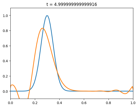
plt.plot(x, qinit(x), x, q, linewidth = 2)
plt.axis((0,1,-0.1,1.1))
plt.title('t = '+str(t))

Text(0.5, 1.0, 't = 4.999999999999916')

Lax Wendroff scheme

Lax and Wendroff’s scheme can be written

\[ q_i^{n+1} = q_i^n-\frac12 \sigma \left( q^n_ {i+1} -q^n_ {i-1} \right) +\frac12 \sigma^2 \left( q^n_ {i+1} -2q^n_ {i}+q^n_ {i-1} \right) \]

With \( \sigma = a \, \delta t/\delta x \)

This diagram is visibly more precise (blatant on dissipation). But there are some oscillations (this may depend on the stiffness of the solution transported.

3. What is the origin of the different terms of this equation? Can we determine the order of precision?

The 1st term is the centered discretization of the transport term (order 2 in expected space). The 2nd term is a distribution term whose intensity is \( a (\delta t)^2\). This term has no reason to be and can only contribute to the error, except that it is necessarily stabilizing. We can however show (not obvious in this form) that the combination of this term with temporal discretization makes it possible to obtain a diagram of order 2 in time.

This scheme can either be generalized in a form of several stages, or include temporal terms in the formulation of the flow. It therefore remains coupled in time and space.

ndof = 100
dx   = 1./ndof                              # cell size
x    = np.linspace(-dx/2.,1+dx/2.,ndof+2)   # cell centers with internal domain + ghost cells (size = ndof+2) 

t   = 0.      # current time (initialized to zero)
dt  = 5e-3    # time step
nit = 1000     # number of iterations

# q[0] is the left ghost cell, q[1] is the first cell, q[ndof] is the last cell, q[ndof+1] is the right ghost cell
# python syntax: q[-1] = q[ndof+1] 
q    = qinit(x)
qnew = q.copy()  # initialize of temporary array

for j in range(nit):
    # periodic boundary conditions
    q[0]  = q[-2]
    q[-1] = q[1]
    # for all internal points
    for i in range(1,ndof+1):
        qnew[i] = q[i] - ( aconv*dt/dx * (q[i+1]-q[i-1]) - (aconv*dt/dx)**2 * (q[i+1]-2*q[i]+q[i-1]) )/2.
    q   = qnew.copy()
    t  += dt
    
plt.plot(x, qinit(x), x, q, linewidth = 2)
plt.axis((0,1,-0.1,1.1))
plt.title('t = '+str(t))

Text(0.5, 1.0, 't = 4.999999999999916')