Introduction

%matplotlib inline
import numpy as np
import matplotlib.pyplot as plt

On cherche à résoudre l’évolution instationnaire du problème linéaire de convection suivant

\[ \frac{\partial q}{\partial t} + a \frac{\partial q}{\partial x} = 0 \]

pour la quantité transportée \(q(x,t)\) et la condition intiale \(q_0(x)\) sur le domaine \([0;\ell]\) avec des conditions périodiques. On choisit \(\ell=1\rm~m\) et \(a=1\rm~m/s\).

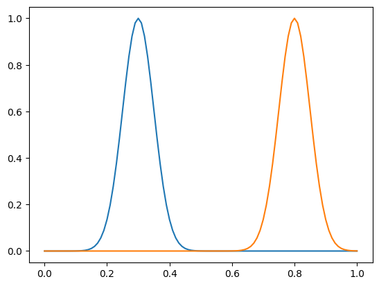
Condition initiale et solution théorique

ndof  = 100
xi    = np.linspace(0,1,ndof+1)  # grid definition
aconv = 1.0                      # Advection velocity

def qinit(x):                 # Initial condition
    q0 = np.exp(-200.*(x-0.3)**2)
    # q0 = .5+.5*np.sin(2*x*np.pi)
    # q0 = .5+.5*np.sin(4*x*np.pi)*(x>.25)*(x<.75)
    return q0

tf = .5 
plt.plot(xi, qinit(xi), xi, qinit(xi-aconv*tf))

[<matplotlib.lines.Line2D at 0x7fb44c131850>,
 <matplotlib.lines.Line2D at 0x7fb44c142bd0>]