Runge-Kutta explicit methods

stability of exponential expansions

Runge-Kutta (RK) methods are a class of numerical methods for solving initial value problems (IVP).

\[ \frac{dQ}{dt} = R(Q) = A\cdot Q \]

One integration step is made of several evaluations of the right-hand side of the ODE, named stages. Each stage uses a set of weights for each previous evaluation of \(R(Q)\). All coefficients can be displayed in the Butcher array.

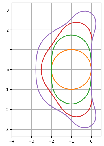
If \(R(Q)\) is linear, the theoretical solution is \(Q_0 \exp(At)\). This is a key argument to show that a k-th order RK method defined by \(Q^{n+1}=P(A\delta t)\cdot Q^n\) should be consistent with the Taylor expansion of \(\exp(A\delta t)\).

import math
import numpy as np
import matplotlib.pyplot as plt

def integrator(order, adt):
    """returns the Taylor expansion of exp(adt) up to order"""
    return np.sum([1./math.factorial(k) * adt**k for k in range(order+1)], axis=0)

fig, ax = plt.subplots(figsize=(4, 6))
cmap = plt.get_cmap('tab10')
x = np.r_[-4:.5:30j]
y = np.r_[-3:3:60j]
X, Y = np.meshgrid(x, y)
adt = X+Y*1j
#
ax.axis('equal')
ax.grid()
for order in range(1, 5):
    ax.contour(X, Y, abs(integrator(order, adt)), levels=[1], linewidths=2, colors=[cmap(order)]) # contour() accepts complex values

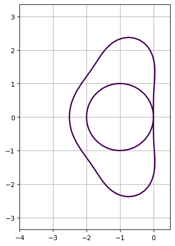
Butcher arrays

Instead of using expected properties of the expansion of the propagator, we can actually use the multi-stage definition of RK method to be able to compute actual steps or the equivalent mapping of complex values.

class integrator():
    _butcher = np.array([[0.]])
    _weights = np.array([1.])

    def __init__(self):
        self._nstage = len(self._weights)
        assert self._butcher.shape == (self._nstage, self._nstage)

    def propagator(self, zarray):
        z = zarray.flatten()
        R = 1 + z[:, None] * np.dot(self._weights, np.linalg.inv(np.eye(self._nstage)-z[:, None, None]*self._butcher)@np.ones((self._nstage, 1)))
        return R.reshape(zarray.shape)

fig, ax = plt.subplots(figsize=(4, 6))
cmap = plt.get_cmap('tab10')
x = np.r_[-4:.5:30j]
y = np.r_[-3:3:60j]
X, Y = np.meshgrid(x, y)
adt = X+Y*1j
#
class rk3ssp(integrator):
    _butcher = np.array([ 
        [0.,  0.,  0.],
        [1.,  0.,  0.],
        [.25, .25, 0.] ] )
    _weights = np.array([1.0, 1.0, 4.0]) / 6.0

euler = integrator()
rk3 = rk3ssp()

ax.axis('equal')
ax.grid()
for solver in (euler, rk3):
    ax.contour(X, Y, np.abs(solver.propagator(adt)), levels=[1], linewidths=2) # contour() accepts complex values

error for convection or non-dissipative physics

The integrator on one step \(\delta t\) should represent \(\exp(A\delta t)\). Convection or non-dissipative models are ruled by imaginary eigenvalues. We can then map the integrator on the imaginary axis \(\lambda\) and compare it to the theoretical integrator or propagator \(P(\lambda)\). \(\ln(P(\lambda))\) is then compared to \(\lambda\) as real and imaginary part in order to separate dissipation and dispersion effects of the approximate integrator. Note that for convection problems, \(|\lambda|\delta t\) is the cfl number.

cfl = np.geomspace(5e-2, 5, 100)*1j

fig, (axr, axi) = plt.subplots(1, 2, figsize=(10, 4))
for ax, ylab in zip([axr, axi], ['dissipation error', 'dispersion error']):
    ax.set_xlabel(r"${\rm cfl}=|\lambda|\delta t$") ; ax.set_ylabel(ylab)
    ax.grid()
    ax.set_ylim(1e-5, 2e1)
for solver, label in zip([euler, rk3], ['Euler', 'RK3ssp']):
    err = np.log(solver.propagator(cfl)/np.exp(cfl))
    axr.loglog(abs(cfl), abs(err.real), label=label)
    axi.loglog(abs(cfl), abs(err.imag), label=label)
axr.legend() ; axi.legend();

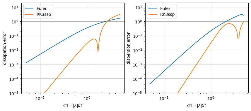
Note

Note that the drop of RK3 method is due to change of sign of dissipative effect. It is then the stability threshold for imaginary eigenvalues.

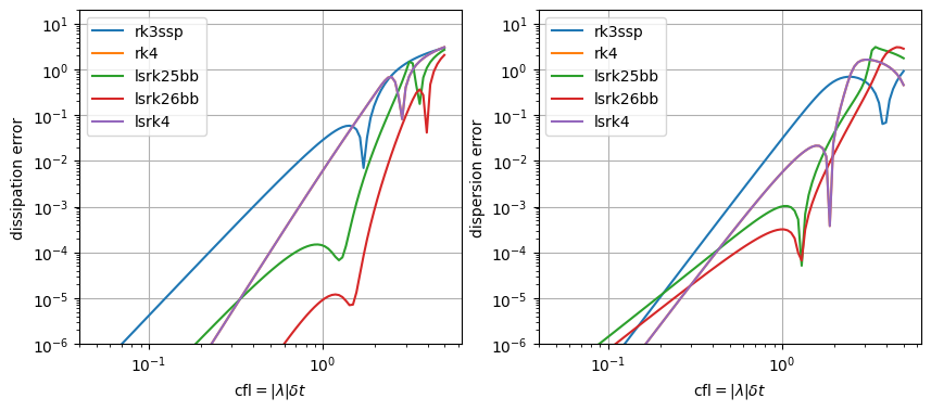
Optimized Runge-Kutta methods

Increasing the number of stage to increase the order of the scheme is the basic idea of Runge-Kutta methods and leads to an unique scheme for linear operators (defined by the expansion of exponential). But It can also be tuned to provide some other parameters that can be tuned to optimize the scheme. As an example, the following RK25 and RK26 (from Bogey and Bailly) are two second order schemes that are optimized for dispersion and dissipation errors.

import numtoolkit.integration as numint
print(numint.all_erk)

cfl = np.geomspace(5e-2, 5, 100)*1j

fig, (axr, axi) = plt.subplots(1, 2, figsize=(10, 4))
for ax, ylab in zip([axr, axi], ['dissipation error', 'dispersion error']):
    ax.set_xlabel(r"${\rm cfl}=|\lambda|\delta t$") ; ax.set_ylabel(ylab)
    ax.grid()
    ax.set_ylim(1e-6, 2e1)
for solvermethod in numint.all_erk:
    solver = solvermethod()
    err = np.log(solver.propagator(cfl)/np.exp(cfl))
    name = solver.__class__.__name__
    print(name)
    axr.loglog(abs(cfl), abs(err.real), label=name)
    axi.loglog(abs(cfl), abs(err.imag), label=name)
axr.legend() ; axi.legend();

[<class 'numtoolkit.integration.rk3ssp'>, <class 'numtoolkit.integration.rk4'>, <class 'numtoolkit.integration.lsrk25bb'>, <class 'numtoolkit.integration.lsrk26bb'>, <class 'numtoolkit.integration.lsrk4'>]
rk3ssp
rk4
lsrk25bb
lsrk26bb
lsrk4